Given
An amplifier topology, its initial state, a technology model, and design targets.
NeurIPS 2026 Poster
1 MIT EECS2 Analog Devices3 IBM Research
A locally deployable 4B language model learns to optimize analog circuits through simulator feedback, with generalization to held-out topologies and unseen technology nodes.
Four-specification Pass@1: gain, −3 dB bandwidth, power, and phase margin. Domain-validity gates and 5% evaluation tolerance apply. One turn evaluates a model-proposed set of parameter updates with a simulator call.
Analog integrated circuit design requires repeated decisions over coupled performance trade-offs, often guided by human intuition and hand-crafted tuning. Learning this expertise from examples alone would require broad design coverage. Yet public circuit data are scarce, and fabrication-process models and many circuit designs are proprietary.
These constraints motivate a small, locally deployable reasoning language model. When confidentiality requirements preclude hosted LLM services, it can keep sensitive circuit and process data in-house while exposing human-interpretable reasoning and interactive parameter updates that engineers can inspect. Compared with purely numerical search, such as Bayesian optimization, this approach also exposes the rationale behind proposed changes and supports an interactive design process.
SLIC combines a small set of demonstrations with reinforcement learning from verifiable simulator feedback. Simulation provides both new experience and a measurable learning signal, enabling a local 4B model to practice successive design decisions without requiring a large proprietary design corpus.
Given an analog amplifier and design targets, adjust the circuit so that it satisfies all targets together. The circuit connectivity is fixed within each task. The model proposes parameter updates, runs a circuit simulator, and uses measured simulation results to decide what to change next.
An amplifier topology, its initial state, a technology model, and design targets.
Which circuit parameters to change, by how much, and how many updates to make before the next simulation.
The simulated circuit meets gain, bandwidth, power, and phase-margin requirements together within the simulator-call budget.
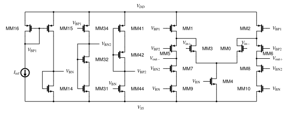
The starting circuit falls short on gain, power, and phase margin. Four turns of parameter updates and simulation produce a design that meets all four targets.
| Specification | Initial | Target | After 4 turns |
|---|---|---|---|
| Gain | 25.0 dB | ≥ 61.7 dB | 68.4 dB |
| Power | 14,349 μW | ≤ 425.7 μW | 318 μW |
| Bandwidth | 111 kHz | ≥ 43.1 kHz | 172 kHz |
| Phase margin | −36.0° | 30–90° | 56.4° |
These objectives are coupled: increasing bias current can improve bandwidth while consuming more power. A useful edit must account for the other requirements, rather than maximize one metric in isolation.
Inspect each turn and its measured outcome ↓A turn is one model response followed by one simulator call. The model chooses a variable number of parameter updates, which are applied together before evaluating the resulting circuit. For example, the first turn above contains 22 parameter updates.
The input is a structured circuit graph represented as text, together with design targets, device parameters, and measured simulation results.
↳ Repeat until success or the simulator-call budget is reachedSupervised fine-tuning teaches a starting behavior. Reinforcement learning develops iterative design strategies.
DeepSeek-V4.1-Flash collects simulator-grounded trajectories on public PTM 65 nm circuits. Qwen3.5-4B learns from selected single-turn examples.
A strong teacher proposes parameter updates and observes the simulated outcomes.
The best-observed performance tuple becomes the trajectory’s target specification.
Retain valid turns from successful episodes and valid, improving turns from unsuccessful ones, each with reasoning.
Source: manuscript Figure 1 and Section 3.1. Simplified SFT data-construction schematic.
6,981 single-turn samples from 1,568 teacher episodes: 6,233 training samples and 748 held-out samples. Episodes are kept separate across the two splits; both cover the same 35 topologies.
Teacher–student analogy. The demonstrations teach a student the basic circuit reasoning, response format, and parameter-update language before it practices making successive decisions on its own.
The SFT-initialized model learns from verifiable simulator feedback over rollouts of up to eight turns.
Sample and simulate alternatives, continue from one eligible state, and retain all candidates for policy learning.
Invalid amplification cannot earn misleading performance credit. Gain and frequency-response checks establish whether the design is meaningful before rewarding its specifications.
Validity and performance signals are normalized separately so that invalid-action penalties do not overwhelm differences among measured designs.
Once all targets are satisfied, additional performance headroom continues to provide a learning signal, even in all-success groups.
Each prompt includes circuit connectivity, design targets, device parameters, operating-point measurements, and admissible actions. Matched devices share parameters. A single interaction turn may contain several parameter changes before the next simulation.
<action>decrease @10 l_MM30 50.0%</action>
<action>increase @70 iref 15.0%</action>
41 amplifier topologies, paired with design targets and initial circuit states. Training uses public PTM 65 nm models and ngspice.
35 amplifier topologies
Design targets + initial states
The same 35 topologies
Separate evaluation tasks
6 topologies held out from training
2 simple + 4 complex
Source: manuscript Table 15, standard task setting.
Seen vs. unseen refers to the topology, not whether an evaluation task was used for training. The paper calls these in-distribution (ID) and out-of-distribution (OOD), respectively.
Success: valid amplifier operation and simultaneous satisfaction of gain, −3 dB bandwidth, power, and phase-margin targets. Unless otherwise stated, Pass@1 uses one rollout per task, a 5% evaluation tolerance, and up to eight simulator calls.
Qwen3.5-4B · trained at PTM 65 nm. One rollout per task, evaluated within the simulator-call budget.
Reinforcement fine-tuning substantially improves circuit optimization over the base and SFT policies. The improvement extends to topologies excluded from training.
840 tasks · 35 training topologies
240 tasks · 6 unseen topologies
Main-policy comparison at the selected interaction budget. Values are mean ± standard deviation over three stochastic evaluation runs per checkpoint. Source: manuscript Tables 1–2.
| Model | Seen topologies (ID) | Unseen topologies (OOD) | Evaluated tasks (ID / OOD) |
|---|---|---|---|
| SLIC–Random (4B) | 87.1 ± 0.7% | 70.6 ± 1.2% | 840 / 240 |
| SLIC–Softmax (4B) | 84.3 ± 1.0% | 72.6 ± 2.0% | 840 / 240 |
| DeepSeek-V4.1-Flash Think | 38.6 ± 1.3% | 26.7 ± 2.2% | 840 / 240 |
| GPT-6-Astra | 90.6% | 86.2% | 840 / 240 · one evaluation run |
All models use the same 840 in-distribution (ID) and 240 out-of-distribution (OOD) tasks. GPT-6-Astra uses one evaluation run with one rollout per task; SLIC and DeepSeek report mean ± standard deviation over three runs. DeepSeek’s ID result aggregates two 420-task batches evaluated at different times (paper Appendix I.2). At four turns, SLIC–Random reaches 74.9% ID success versus Astra’s 67.1%; at eight turns, their scores are 87.1% and 90.6%, respectively.
A policy trained at PTM 65 nm remains effective across five unseen nodes without additional fine-tuning. SLIC–Softmax achieves 61.9–71.0% held-out-topology success across PTM 22, 32, 45, 90, and 130 nm, compared with 72.6% at the training node. The same training process also supports transfer to a commercial foundry PDK, evaluated below.
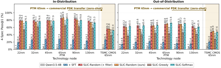
A commercial foundry PDK is a more detailed practical design environment than the public PTM models used for training, even at the same nominal 65 nm node. Further local RL offers a route to adapt the policy to that environment and potentially improve performance; the results above measure transfer before such adaptation.
We extend the evaluation budget to 32 simulator calls and compare policies trained with different rollout horizons. The best-performing variants reach 95.3% success on seen topologies and 83.2% on unseen topologies.
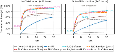
Interpretation. Four-turn training preserves continued improvement at evaluation time, whereas single-turn training saturates earlier. A single-turn training episode provides no experience of revising a design after feedback. These results suggest that a moderate training horizon can retain iterative refinement while reducing training cost.
The gains persist when evaluation requires strict target satisfaction. At 0% tolerance, SLIC–Random reaches 71.9% ID success and SLIC–Softmax reaches 59.3% OOD success. Across the 0–15% evaluation sweep, Random trained with the default 5% success tolerance outperforms its zero-tolerance training counterpart, including at strict 0% evaluation.
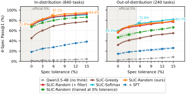
Interpretation. Modest training tolerance may make successful outcomes easier to reach early in learning, while the success-conditional slack bonus continues to encourage headroom.
Greedy develops the longest responses but remains less successful than Random and Softmax. Response length alone is therefore an incomplete indicator of effective use of simulator feedback.
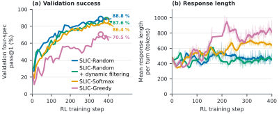
Observation. More generated reasoning does not necessarily yield better circuit refinement. In the sampled responses, Greedy repeatedly reconsiders its decisions, while Softmax more often connects simulator feedback to a diagnosis, proposed updates, and expected effects.
Two recorded SLIC–Random rollouts show recovery from invalid operation and refinement toward all four targets.
Bias-generation circuitry (left) and folded-cascode amplifier core (right). Device identifiers match the recorded actions.
Choose Turn 1–4 to inspect the model’s parameter updates.
Verbatim model excerpt. It can contain numerical or physical errors; outcomes are assessed from simulator measurements.
Choose Turn 1–4 to read the recorded excerpt.
Source: manuscript Appendix L.1–L.2; schematics correspond to Figures 11–12. Both examples satisfy the original four targets after four turns without relying on the 5% evaluation tolerance. The displayed targets are nominal; invalid states are never counted as successful. Full case studies · Coming soon
Public paper, code, and benchmark links will be added as they become available. Recorded circuit examples are available on this page.
@inproceedings{xu2026slic,
  title = {SLIC: Reinforcement Fine-Tuning Small LMs for
           Multi-Turn Analog Circuit Optimization},
  author = {Xu, Yan and Gao, Zhengqi and Ko, Ching-Yun and
            Hong, Zhang-Wei and Lu, Wenjie and Yu, Tao and
            Zhang, Xin and Boning, Duane S. and Han, Ruonan},
  booktitle = {Advances in Neural Information Processing Systems},
  year = {2026}
}
Accepted-paper citation; final proceedings metadata and public links are pending.